Introduction
Embedded design and especially design work utilising low speed serial signalling is one of the fastest growing areas of digital electronics design. The need to communicate between modules, FPGAs, and processors within a wide array of consumer and industrial electronics is increasing at an astounding rate. Customised communication protocol and bus usage is critical to design efficiency and time to market, but comes with the risk of being sometimes difficult to analyse and debug. The most common sources and types of problems when using low speed serial data in an embedded application include timing, noise, signal quality, and data. We will recommend debug tips and features available in modern oscilloscopes that will make debugging these complex systems faster and easier.
Types of Errors
Timing
Timing is critical in any serial data system, but finding the system timing limitations related to components, transmission length, processing time, and other variables can be difficult. Let’s start with a simple 16 bit DAC circuit. First, make sure you understand the data and timing specifications for the protocol in use. Does it sample data right on the clock edge? How far off can the clock and data be when we still expect good data? In other words: do we have a clock sync error budget defined? Once we understand these timing requirements then we can experimentally verify both the Tx and Rx hardware subsystems. Now we can analyse the system level timing delays and the overall accuracy of the conversions because we can make direct measurements of both the logic and analogue channels in a time correlated fashion. We will also be able to simultaneously view the decoded bit patterns numerically on an oscilloscope that comes in well below your budget limits.
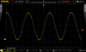
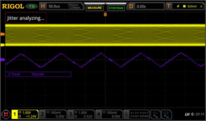
Here is a simple example of measuring a bit on channel 2 (blue) that is driving the DAC output that is creating the Sine wave on channel 1 (yellow).
Utilising parallel bus decoding (Figure 1) we can get a quick look at the transitions of this single line. But this doesn’t give us all the information we need since the DAC is utilising a number of data lines to set its output level. Getting more complete data requires a different approach. Let’s move all the DAC lines (Figure 2) over to the MSO’s digital inputs. Now we can see how the digital lines really coordinate with the DAC output. To investigate further we can simplify the decoding to show Hex values (Figure 3) and zoom in so we can view the decoded data.
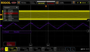
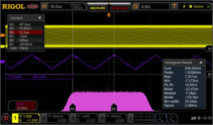
Now we can use the zoom feature to clearly see the relationship between the bit and DAC transitions (Figure 4). For the zoom we have turned on analogue channel 2 in blue that is on the DAC clock. Zoomed in by a factor of 500x from 50 usec per division to 100 nsec per division allows us to see that the bit transitions are occurring 100 nsec before the clock transition. The clock transitions in under 5 nsec and the DAC output starts changing in sync with the clock. We can also utilise the scope cursors to make the timing in the transitions clearer and well defined (Figure 5).
Verifying timing in mixed signal systems can be made easier with the right tools. Select a modern scope with the correct set of channels and options to make sure you can easily view what you need on the display when you need it. From digital buses to processing delays, get the full picture of the device’s operation and delve into details as needed to verify timing issues on your device.
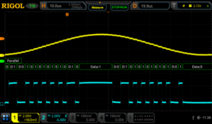
Figure 1: DAC output and input bit on a RIGOL MSO5354 Digital Oscilloscope
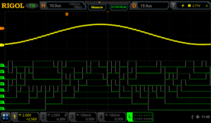
Figure 2: DAC output and 8 bit input bus on a RIGOL MSO5354 Digital Oscilloscope
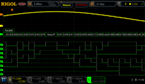
Figure 3: DAC output and 8 bit input bus with Hex decode on a RIGOL MSO5354 Digital Oscilloscope
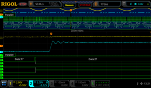
Figure 4: DAC output and 8 bit input bus zoomed in on a RIGOL MSO5354 Digital Oscilloscope
We can also trigger on the digital patterns instead of the analogue signal (Figure 6). Triggering on a digital pattern can be critical for debugging when there is a problem. There isn’t always a good way to track events from the analogue side of a system. When using a digital trigger method make sure to set the additional trigger parameters. These may include start bits or even address and data for some protocols. Even for a simple parallel bus like this you need to define and arrange the channels in the bus for the results to be easiest to interpret.
Accurate timing of Low Speed Serial signals is critical to system stability. Therefore, making sure your measurement tools are up to the task of precise and easy triggering, monitoring, and analysing of your waveforms is vital to improved R&D efficiency and ultimately time to market.
Noise
One of the most common issues in correct serial data measurements is the handling of system noise. Noise in these measurements can come from a number of sources including poor grounding, bandwidth issues, crosstalk, electromagnetic immunity (EMI) problems. Sometimes the problem is in the device, but improved probing and measurement techniques can also improve the results significantly without changing the device under test. A good first step is always to make sure we are using best measurement practices.
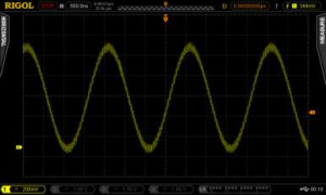
Here is a decoded I2C bus segment using a 5000 series oscilloscope (Figure 7). In the first example we have extremely poor grounding on our probes. Because the scope’s ground is tied directly to power ground signals that need to float or simply use a different or noisy ground plane can cause results like this. It is also possible for high current draw through ground in local power to create ground loops that can cause noise to be injected in your system. We solve these problems in order from easy to difficult. First, we can look at our probe connections. Normally, we would use the alligator clip ground strap that connects on the probe to make a ground connection. Assuming we are doing that correctly and still having a problem we may need to use the ground spring instead. The ground spring connects closer to the probe tip and significantly reduces the loop area of the connection. This can significantly improve noise and signal quality (Figure 8) especially for high speed signals or signals sensitive to capacitance or coupled voltages.
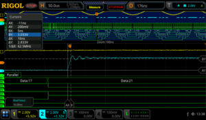
Figure 5: DAC output and 8 bit input bus zoomed in with cursors shown on a RIGOL MSO5354 Digital Oscilloscope

Figure 6: DAC output and 8 bit input bus triggered by a digital pattern on a RIGOL MSO5354 Digital Oscilloscope
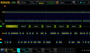
Figure 7: I2C clock and data with noise from poor grounding in a colour graded display using a RIGOL MSO5354 Digital Oscilloscope
Figure 8: I2C clock and data with ground noise improved in a colour graded display using a RIGOL MSO5354 Digital Oscilloscope
All RIGOL probes come with both the standard ground strap and the ground spring for these types of measurements.
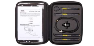
If ground noise is still an issue, try isolating your device from ground. The scope operates best grounded to AC power ground via the plug. If the rest of the device or system being tested can be isolated from ground this eliminates ground loops. If ground noise is still an issue you may consider a differential probe like the RP1100D (Figure 9) which enables measurements without reference to ground on the scope. Differential measurements may be the only way to clearly view some low speed serial data such as a LVDS bus (Low Voltage Differential Signalling). Buses like this purposely move the reference line to maximise bandwidth and increase communication distances, but it may require true differential probing or the use of multiple channels of your scope together to view the signal correctly. RIGOL has several different probe types for these measurements including the RP1000D series differential probes typically used for high voltage floating applications and the RP7150 1.5 GHz differential probe (Figure 10) for high speed data applications.
Now that we have improved our signal to noise ratio by decreasing noise injected from the ground, we can turn our attention to bandwidth filtering. High frequency noise can also enter your measurements via channel to channel cross talk or other high frequency sources nearby or within your
device. One way to address this is to utilise the channel bandwidth limits (Figure 11). Every RIGOL scope channel can limit the bandwidth to the ADC. A 20 MHz limit is pretty standard. Some scopes will have higher options as well.
Additionally, there are a few acquisition mode and triggering settings that can improve performance in the face of noise. Many trigger types have a menu item allowing you to turn on noise rejection for the triggering scheme. The 5000 series even includes HFR and LFR (high and low frequency rejection) as options in how to couple the signal triggered on. The 5000 series comes with High Res or High Resolution mode (Figure 12). This feature uses extra oversampling that is being done behind the scenes on many measurements to provide an average that results in less noise. This is best to use if you are able to set the sampling to take at least 200 samples per time division. This will average rather than reject high frequency signals, so be sure to understand your potential error sources and how they may interact with your measurement setup. Finally, the 5000 series scope also has an NRJ (noise reject) feature directly within the trigger menu. This removes noise that appears in bursts and can be set in time rather than frequency.
To further isolate and locate sources of noise within your system you may want to focus on EMC or EMI related issues. To further investigate these error sources please download the EMC Precompliance app note for use with the Rigol DSA815 Spectrum Analyser at http://www.rigolna.com/EMC
Noise is always a concern when working with low speed serial signals. By definition these signals continue to go to higher speeds, more advanced encoding, farther transmission distances, and lower voltage and power levels. All of these trends make hardware more susceptible to noise. Making careful measurements that limit or eliminate adding noise to our system then enables us to focus on noise in the system that may still cause long term design issues.
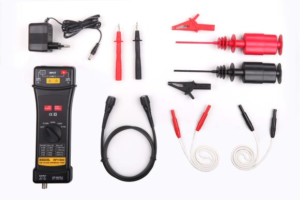
Figure 9: RP1100D 100 MHz Differential Probe
Figure 10: RP7150 1.5 GHz Differential Probe
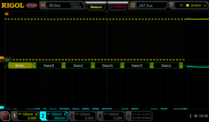
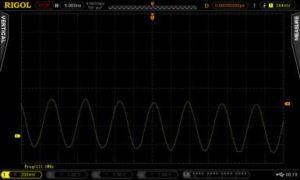
Figure 11: I2C clock data with reduced noise using bandwidth limit on a RIGOL MSO5354 Digital Oscilloscope
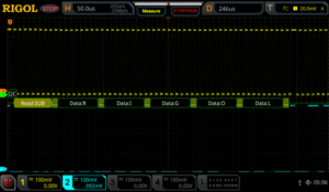
Figure 12: I2C clock and data using high resolution mode on a RIGOL MSO5354 Digital Oscilloscope
Signal Quality
Monitoring and improving the quality of low speed serial signals is a critical part of the debugging process. Issues like impedance mismatches, bandwidth, and loading errors can all effect the quality of signals even when noise isn’t present. Now that we are looking more closely at the exact nature of these signals it is important to verify the way we are using our oscilloscope for these tests. For signal quality tests we will be using the analogue channels because they provide the best look at what is actually occurring with our signals. This requires some additional forethought. To clearly see data transitions, we should definitely use a sampling rate that is as high as possible. Sampling at 5x the bit rate of the digital bus should be considered the minimum because of the high frequency components that we need to visualise. Sampling at 10 times the bit rate should enable us to see
any of the issues. But when we decode the signal the scope likely uses a subset of the full memory data to handle the decode analysis. This can be important because you don’t necessarily want to decode being performed at too high of a rate. That can mask problems you will find when a more nominal receiver is used to decode the data. On RIGOL scopes the decode is done on 1 Mpts of memory spread across the acquisition. By setting the memory depth and the time per division the user can determine whether they want the decode to be done directly from the analogue points or from a subset. Decoding is also shown across the display region. To capture more decoded bytes than you can view on the display use the event table function (Figure 13). You can also export the table results to a text file from the event table menu for record keeping or offline timing analysis.
Here is an example table of how the memory depth, time per division, and sample rate effect the actual decode sample rate on a MSO5000 Series. Based on your serial data speeds and the receiver you will eventually use to collect the serial data you can optimise your serial decode rate.
Now that we have set and verified our sampling times for best analogue and decoding results, we also want to set our display up for optimal triggering conditions. When triggering on the rising edge of an analogue signal make sure to keep the trigger level at least 1 division away from the signal low state. This separation allows for consistent
triggering action without any false triggers. When visualising digital signals with the analogue channels use more screen real estate when possible. Using about 2 vertical divisions and about ½ to 1 horizontal division per decode character will allow you to see any major overshoot or impedance issues as well as some of the other types of error we will be looking at. Here is the setup (Figure 14) I prefer to monitor decoded data on a bus like RS232.
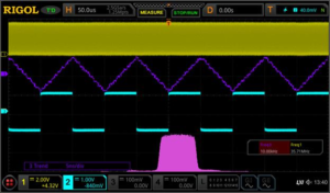
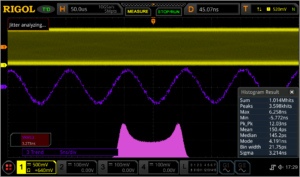
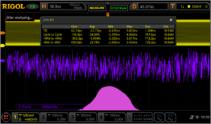
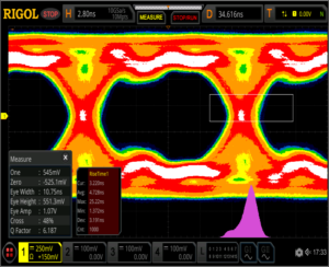
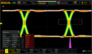
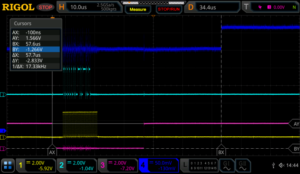
On a more complex bus like I2C we view both clock and data lines on the screen. The timing correlation between multiline buses is, of course, vital to successful decoding. Making critical measurements on the screen like risetime and overshoot for each line makes reliability tests simple to setup. We can view the measurements in max/min or using standard deviation notation for more advanced statistical testing (Figure 15).
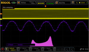
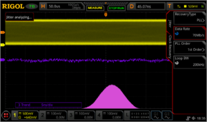
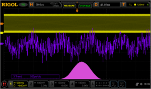
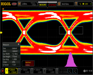
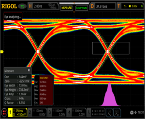
In addition to the risetime and overshoot for the 4 serial bus lines you can also see the jitter in the clock when compared to the data transition. This test device appears to have the clock transition occur about 1.6 microseconds of jitter on the clock when viewed, as above, in reference to the triggering data transition. In (Figure 16) we zoom in on the data transition to get a more accurate measurement of the risetime and overshoot.
Signal quality encompasses many of the types of issues you find on LSS buses. Efficient debug means making the most of your embedded analysis capabilities to find signal discrepancies that can lead you to design changes as early as possible in your design process. A mixed signal oscilloscope is the perfect tool for measuring signal quality (Figure 17) from risetime variance to ASCII packet data.
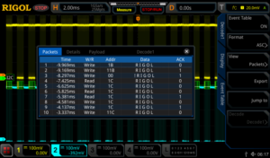
Figure 13: I2C clock and data event table view using a RIGOL MSO5354 Digital Oscilloscope
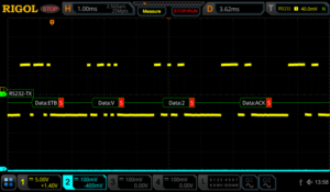
Figure 14: RS232 optional decoded data view settings using a RIGOL MSO5354 Digital Oscilloscope
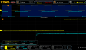
Figure 15: I2C clock and data min/max signal measurements using a RIGOL MSO5354 Digital Oscilloscope
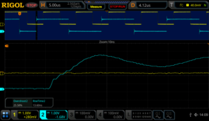
Figure 16: I2C zoom in on data risetime measurement using a RIGOL MSO5354 Digital Oscilloscope
Data
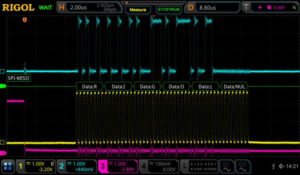
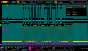
The key to any Low Speed Serial application is the ability to quickly and easily look at the data being transmitted. This means adding the capability to do embedded decoding on your oscilloscope. Decoding affects both the triggering and display on the scope. It adds a decoded bus display to the instrument’s screen. You can decode values as ASCII or as hex, octal, or binary data depending on what you want to look at. You can also trigger on these values to make sure you are looking at the packets of most interest to you (Figure 18). In addition to triggering on these signals with the decode specific trigger you are also able to trigger on any type of signal with a zone trigger which allows you to not only to trigger on any type of signal but also exclude any unwanted noise or data from a signal. These are created by simply drawing a rectangle on the screen of the instrument (Figure 19).
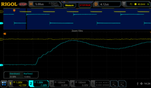
Figure 17: I2C data measurements with standard deviation using a RIGOL MSO5354 Digital Oscilloscope
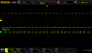
Figure 18: RS232 optimal decoded data view settings using a RIGOL MSO5354 Digital Oscilloscope
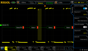
Figure 19: A zone trigger is added to exclude part of the RS232 signal.
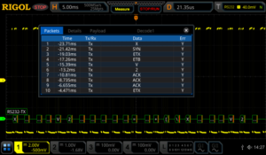
Figure 20: RS232 event table capture of multiple transmissions using a RIGOL MSO5354 Digital Oscilloscope
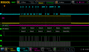
If you are interested in timing between packets or evaluating more than one or two consecutive packets of data, use the event table mode (Figure 20) to generate a list of data packets on a wider time base. Additionally, with using an event table you are easily able to move around on the decoded signal by stopping the instrument from sampling and then select your desired trigger point in the packet’s submenu on the event table then press the Jump To button to move to the desired trigger point on the captured signal (Figure 21).
You can always utilise the zoom function to see the signals and data from an individual packet in that series (Figure 22).
Another way to view this signal is by using the search and navigation menu. This allows you to view multiple trigger points and easily move around on the signal when the scope has stopped scanning. All of the trigger points are represented on the search and navigation menu and they correspond to the white triangles at the top of the screen. The trigger point that is highlighted on the table corresponds with the red triangle at the top of the screen (Figure23).
To view how decoded segments, differ over time or compare between triggered events when other signals might be affecting the results the best analysis method is often to use record mode. RIGOL’s record mode enables you to capture thousands of frames around a trigger event. Once captured, you can use pass/fail or a trace difference analysis mode to visualise changes from frame to frame (Figure 24).
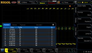
Figure 21: RS232 Event used to move around on the signal by using the Jump To soft key.
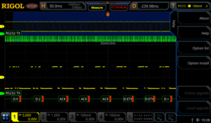
Figure 22: RS232 packet view using zoom mode on a RIGOL MSO5354 Digital Oscilloscope
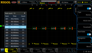
Figure 23: Using Search and Navigation feature to move around on the RS232 signal.
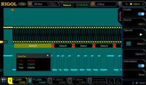
Figure 24: I2C with pass/fail analysis enabled using a RIGOL MSO5354 Digital Oscilloscope
These recordings can be stored and played back as a movie as well, but the analysis features let you search for failures or outliers while also viewing decoded data for comparison (Figure 25).
Data errors as well as the debugging process are always closely tied to the protocol and its specifications. To be efficient with your test equipment make sure you are utilising the best analysis method to easily view the data you need to see without extraneous results getting in your way.
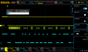
Figure 25: I2C transmission record mode in playback using a RIGOL MSO5354 Digital Oscilloscope
Keys to Look Out For
Proper Oversampling & Bandwidth
As discussed, proper sampling is critical to making correct measurements as well as completely debugging your low speed serial signal. A good rule of thumb for analogue signals is 5x the bandwidth of the signal you want to measure. This limits your risetime error to about 2%. To view the best detail on high frequency signal components set up your scope to achieve 5-10X over sampling as well. When digital signals this means sampling 5 times in the width of one bit. When sampling on digital lines or for sampling that will be used for decoding oversampling is less important but set up your measurement device so it is as similar as the LSS receiver you will ultimately be using. This gives you the best chance to focus on material errors that will cause problems down the road.
Grounding, Noise, and Differential Signalling Proper probing and understanding the use of
differential vs. ground referenced signals is important to debugging. If your data lines are not ground referenced make sure to understand the impact of ground loops and ground coupled noise on your measurements. Use proper probe techniques and advanced noise cancelling features on the scope to limit noise sources. If necessary, add differential probes to your measurement system to improve measurement quality.
How to Best View Low Speed Serial Signals There are a number of methods for analysing,
viewing, and evaluating LSS bus activity on a modern oscilloscope. The best way differs depending on whether you want to look at a single bit transition for noise, speed, or synchronization; whether you want to look at a complete packet of data; or if you want to compare packets and packet timing over a longer time period. Make sure your bench tools allow you to see everything you need and familiarise yourself with features like zoom, record mode, search and navigation, event tables, deep memory, and automatic measurements as well as how they interact and how best to transition between them when considering your test plan. Ideally, an oscilloscope empowers you to view all the results you need and quickly switch modes to acquire additional information.
Conclusions
Embedded design and debugging of digital data is a growing test requirement in a broad range of consumer and industrial applications. Having the right mixed signal oscilloscope can make viewing, analysing, and resolving issues including timing, noise, signal quality, and data easier and faster. This improves engineering efficiency and time to market. RIGOL’s line of UltraVision II enabled oscilloscopes comes with standard or optional capabilities for the methods and measurements discussed here and are powerful benchtop instruments that provide uncompromising performance at unprecedented value.
Products Mentioned In This Article:
- DSA815 please see HERE
- MSO5000 Series please see HERE
- RP7150 please see HERE